How we built a derivatives exchange with BigQuery ML for Google Next ‘18
Matt Tait
Technical Solutions Consultant, Google Cloud
Salvatore Sferrazza
Solutions Architect
Financial institutions have a natural desire to predict the volume, volatility, value or other parameters of financial instruments or their derivatives, to manage positions and mitigate risk more effectively. They also have a rich set of business problems (and correspondingly large datasets) to which it’s practical to apply machine learning techniques.
Typically, though, in order to start using ML, financial institutions must first hire data scientist talent with ML expertise—a skill set for which recruiting competition is high. In many cases, an organization has to undertake the challenge and expense of bootstrapping an entire data science practice. This summer, we announced BigQuery ML, a set of machine learning extensions on top of our scalable data warehouse and analytics platform. BigQuery ML effectively democratizes ML by exposing it via the familiar interface of SQL—thereby letting financial institutions accelerate their productivity and maximize existing talent pools.
As we got ready for Google Cloud Next London last October, we decided to build a demo to showcase BigQuery ML’s potential for the financial services community. In this blog post, we’ll walk through how we designed the system, selected our time-series data, built an architecture to analyze six months of historical data, and quickly trained a model to outperform a 'random guess' benchmark—all while making predictions in close to real time.
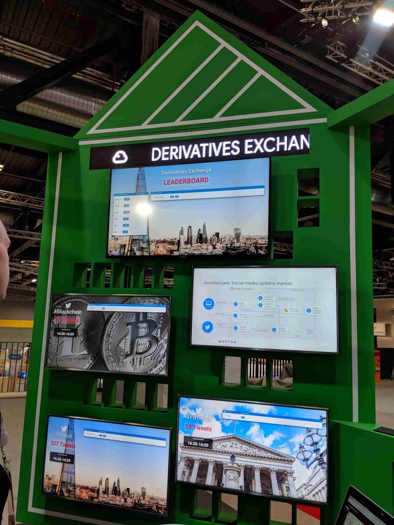
Meet the Derivatives Exchange
A team of Google Cloud solution architects and customer engineers built the Derivatives Exchange in the form of an interactive game, in which you can opt to either rely on luck, or use predictions from a model running in BigQuery ML, in order to decide which options contracts will expire in-the-money. Instead of using the value of financial instruments as the “underlying” for the options contracts, we used the volume of Twitter posts (tweets) for a particular hashtag within a specific timeframe. Our goal was to show the ease with which you can deploy machine learning models on Google Cloud to predict an instrument’s volume, volatility, or value.
Our primary goal was to translate an existing and complex trading prediction process into a simple illustration to which users from a variety of industries can relate. Thus, we decided to:
- Use the very same Google Cloud products that our customers use daily.
- Present a time-series that is familiar to everyone—in this case, the number of hashtag Tweets observed in a 10-minute window as the “underlying” for our derivative contracts.
- Build a fun, educational, and inclusive experience.
When designing the contract terms, we used this Twitter time-series data in a manner similar to the strike levels specified in weather derivatives.
Architectural decisions
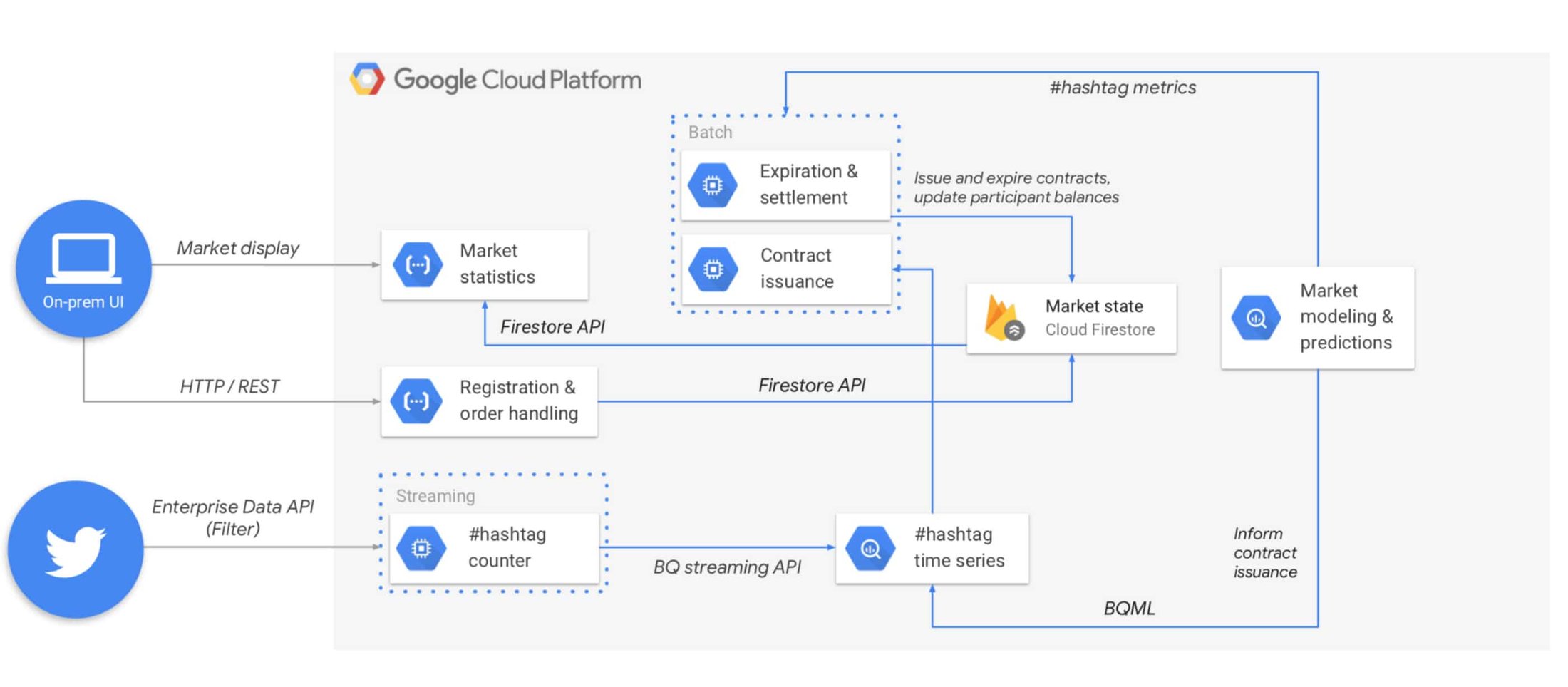
We imagined the exchange as a retail trading pit where, using mobile handsets, participants purchase European binary range call option contracts across various social media single names (what most people would think of as hashtags). Contracts are issued every ten minutes and expire after ten minutes. At expiry, the count of accumulated #hashtag mentions for the preceding window is used to determine which participants were holding in-the-money contracts, and their account balances are updated accordingly. Premiums are collected upon opening interest in a contract, and are refunded if the contract strikes in-the-money. All contracts pay out 1:1.
We chose the following Google Cloud products to implement the demo:
Compute Engine served as our job server:
The implementation executes periodic tasks for issuing, expiring, and settling contracts. The design also requires a singleton process to run as a daemon to continually ingest tweets into BigQuery. We decided to consolidate these compute tasks into an ephemeral virtual machine on Compute Engine. The job server tasks were authored with node.js and shell scripts, using cron jobs for scheduling, and configured by an instance template with embedded VM startup scripts, for flexibility of deployment. The job server does not interact with any traders on the system, but populates the “market operational database” with both participant and contract status.
Cloud Firestore served as our market operational database:
Cloud Firestore is a document-oriented database that we use to store information on market sessions. It serves as a natural destination for the tweet count and open interest data displayed by the UI, and enables seamless integration with the front end.
Firebase and App Engine provided our mobile and web applications:
Using the Firebase SDK for both our mobile and web applications’ interfaces enabled us to maintain a streamlined codebase for the front end. Some UI components (such as the leaderboard and market status) need continual updates to reflect changes in the source data (like when a participant’s interest in a contract expires in-the-money). The Firebase SDK provides concise abstractions for developers and enables front-end components to be bound to Cloud Firestore documents, and therefore to update automatically whenever the source data changes.
Choosing App Engine to host the front-end application allowed us to focus on UI development without the distractions of server management or configuration deployment. This helped the team rapidly produce an engaging front end.
Cloud Functions ran our backend API services:
The UI needs to save trades to Cloud Firestore, and Cloud Functions facilitate this serverlessly. This serverless backend means we can focus on development logic, rather than server configuration or schema definitions, thereby significantly reducing the length of our development iterations.
BigQuery and BigQuery ML stored and analyzed tweets
BigQuery solves so many diverse problems that it can be easy to forget how many aspects of this project it enables. First, it reliably ingests and stores volumes of streaming Twitter data at scale and economically, with minimal integration effort. The daemon process code for ingesting tweets consists of 83 lines of Javascript, with only 19 of those lines pertaining to BigQuery.
Next, it lets us extract features and labels from the ingested data, using standard SQL syntax. Most importantly, it brings ML capabilities to the data itself with BigQuery ML, allowing us to train a model on features extracted from the data, ultimately exposing predictions at runtime by querying the model with standard SQL.
BigQuery ML can help solve two significant problems that the financial services community faces daily. First, it brings predictive modeling capabilities to the data, sparing the cost, time and regulatory risk associated with migrating sensitive data to external predictive models. Second, it allows these models to be developed using common SQL syntax, empowering data analysts to make predictions and develop statistical insights. At Next ‘18 London, one attendee in the pit observed that the tool fills an important gap between data analysts, who might have deep familiarity with their particular domain’s data but less familiarity with statistics; and data scientists, who possess expertise around machine learning but may be unfamiliar with the particular problem domain. We believe BigQuery ML helps address a significant talent shortage in financial services by blending these two distinct roles into one.
Structuring and modeling the data
Our model training approach is as follows:
- First, persist raw data in the simplest form possible: filter the Twitter Enterprise API feed for tweets containing specific hashtags (pulled from a pre-defined subset), and persist a two-column time-series consisting of the specific hashtag as well as the timestamp of that tweet as it was observed in the Twitter feed.
- Second, define a view in SQL that sits atop the main time-series table and extracts features from the raw Twitter data. We selected features that allow the model to predict the number of tweet occurrences for a given hashtag within the next 10-minute period. Specifically:
- #Hashtag
#fintech may have behaviors distinct from #blockchain and distinct from #brexit, so the model should be aware of this as a feature.
- Day of week
Sunday’s tweet behaviors will be different from Thursday’s tweet behaviors.
- Specific intra-day window
We sliced a 24-hour day into 144 10-minute segments, so the model can inform us on trend differences between various parts of the 24-hour cycle.
- Average tweet count from the past hour
These values are calculated by the view based upon the primary time-series data.
- Average tweet velocity from the past hour
To predict future tweet counts accurately, the model should know how active the hashtag has been in the prior hour, and whether that activity was smooth (say, 100 tweets consistently for each of the last six 10-minute windows) or bursty (say, five 10-minute windows with 0 tweets followed by one window with 600 tweets).
- Tweet count range
This is our label, the final output value that the model will predict. The contract issuance process running on the job server contains logic for issuing options contracts with strike ranges for each hashtag and 10-minute window (Range 1: 0-100, Range 2: 101-250, etc.) We took the large historical Twitter dataset and, using the same logic, stamped each example with a label indicating the range that would have been in-the-money. Just as equity option chains issued on a stock are informed by the specific stock’s price history, our exchange’s option chains are informed by the underlying hashtag's volume history.
Train the model on this SQL view. BigQuery ML makes model training an incredibly accessible exercise. While remaining inside the data warehouse, we use a SQL statement to declare that we want to create a model trained on a particular view containing the source data, and using a particular column as a label.Finally, deploy the trained model in production. Again using SQL, simply query the model based on certain input parameters, just as you would query any table.
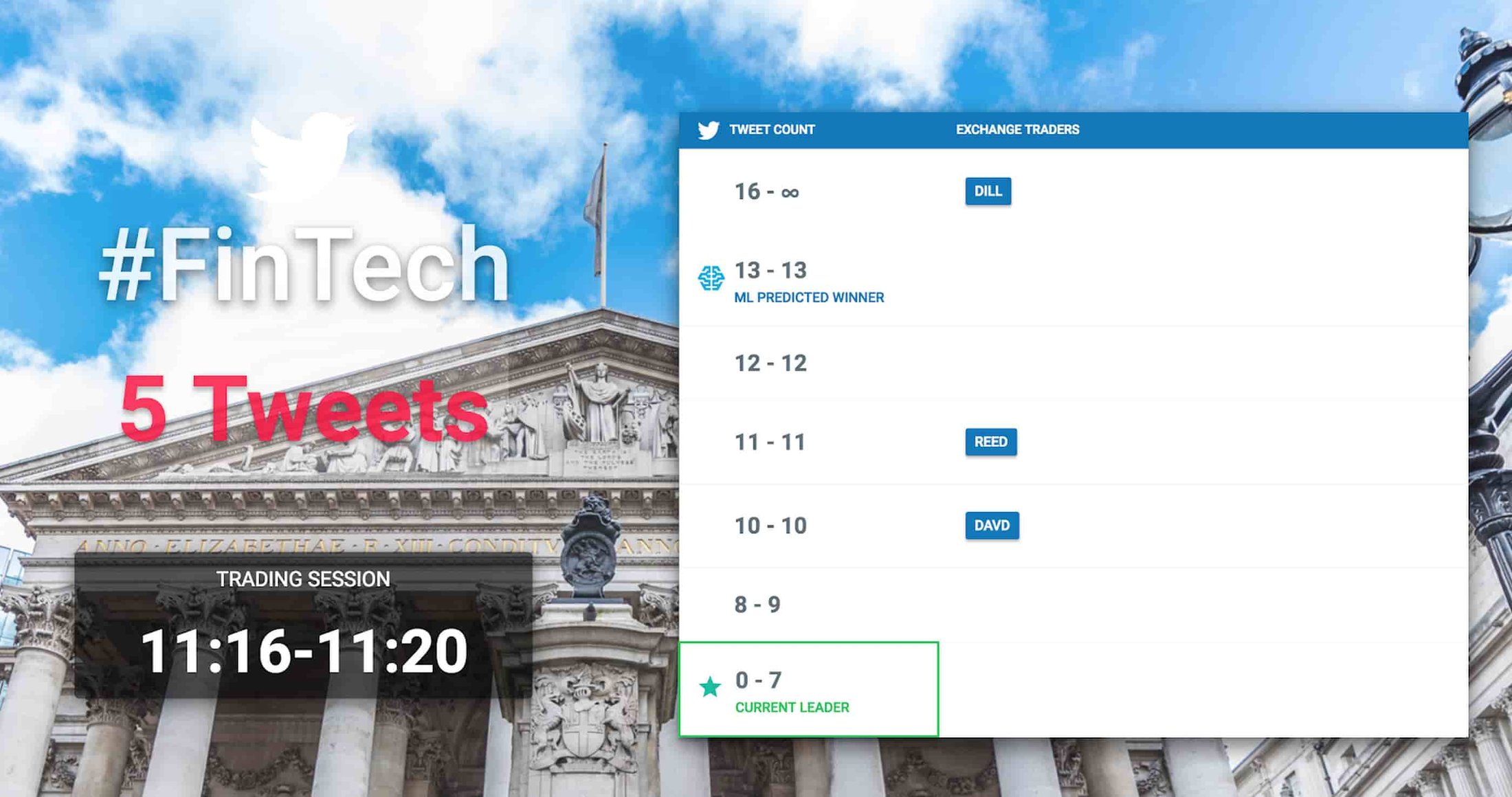
Trading options contracts
To make the experience engaging, we wanted to recreate a bit of the open-outcry pit experience by having multiple large “market data” screens for attendees (the trading crowd) to track contract and participant performance. Demo participants used Pixel 2 handsets in the pit to place orders using a simple UI, from which they could allocate their credits to any or all of the three hashtags. When placing their order, they chose between relying on their own forecast, or using the predictions of a BigQuery ML model for their specific options portfolio, among the list of contracts currently trading in the market. Once the trades were made for their particular contracts, they monitored how their trades performed compared to other “traders” in real-time, then saw how accurate the respective predictions were when the trading window closed at expiration time (every 10 minutes).
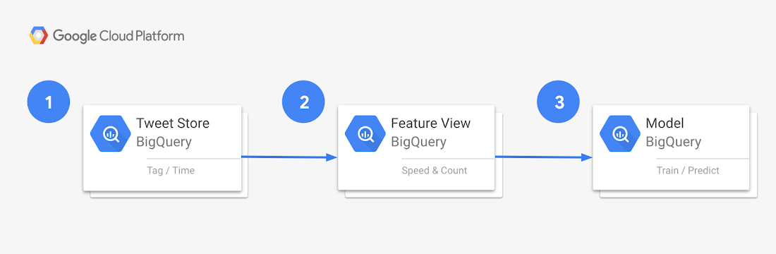
ML training process
In order to easily generate useful predictions about tweet volumes, we use a three-part process, First, we store tweet time series data to a BigQuery table. Second, we layer views are layered on top of this table to extract the features and labels required for model training. Finally, we use BigQuery ML to train and get predictions from the model.
The canonical list of hashtags to be counted is stored within a BigQuery table named “hashtags”. This is joined with the “tweets” table to determine aggregates for each time window.
Example 1: Schema definition for the “hashtags” table
The tweet listener writes tags, timestamps, and other metadata to a BigQuery table named “tweets” that possesses the schema listed in example 2:
Example 2: Schema definition for the “tweets” table
The lowest-level view calculates the count of each hashtag’s occurrence, per intraday window. The mid-level view extracts the features mentioned in the above section (“Structuring and modeling the data”). The top-level view then extracts the label (i.e., the “would-have-been in-the-money” strike range) from that time-series dat
a. Lowest-level view
The lowest-level view is defined by the SQL in example 3. The view definition contains logic to aggregate tweet history into 10-minute buckets (with 144 of these buckets per 24-hour day) by hashtag.
Example 3: low-level view definition
The selection of some features (for example: hashtag, day-of-week or specific intraday window) is straightforward, while others (such as average tweet count and velocity for the past hour) are more complex. The SQL in example 4 illustrates these more complex feature selections.
Example 4: intermediate view definition for adding features
Having selected all necessary features in the prior view, it’s time to select the label. The label should be the strike range that would have been in-the-money for a given historical hashtag and ten-minute-window. The application’s “Contract Issuance” batch job generates strike ranges for every 10-minute window, and its “Expiration and Settlement” job determines which contract (range) struck in-the-money. When labeling historical examples for model training, it’s critical to apply this exact same application logic.
Example 5: highest level view
3. Train and get predictions from model
Having created a view containing our features and label, we refer to the view in our BigQuery ML model creation statement:
Example 6: model creation
Then, at the time of contract issuance, we execute a query against the model to retrieve a prediction as to which contract will be in-the-money.
Example 7: SELECTing predictions FROM the mode
Improvements
The exchange was built with a relatively short lead time, hence there were several architectural and tactical simplifications made in order to realistically ship on schedule. Future iterations of the exchange will look to implement several enhancements, such as:
Introduce Cloud Pub/Sub into the architecture
Cloud Pub/Sub is an enabler for refined data pipeline architectures, and it stands to improve several areas within the exchange’s solution architecture. For example, it would reduce the latency of reported tweet counts by allowing the requisite components to be event-driven rather than batch-oriented.
Replace VM `cron` jobs with Cloud Scheduler
The current architecture relies on Linux `cron`, running on a Compute Engine instance, for issuing and expiring options contracts, which contributes to the net administrative footprint of the solution. Launched in November of last year (after the version 1 architecture had been deployed), Cloud Scheduler will enable the team to provide comparable functionality with less infrastructural overhead.
- Reduce the size of the code base by leveraging Dataflow templates
- Expand the stored attributes of ingested tweets
Storing the geographical tweet origins and the actual texts of ingested tweets could provide a richer basis from which future contracts may be defined. For example, sentiment analysis could be performed on the Tweet contents for particular hashtags, thus allowing binary contracts to be issued pertaining to the overall sentiment on a topic.
- Consider BigQuery user-defined functions (UDFs) to eliminate duplicate code among batch jobs and model execution
Certain functionality, such as the ability to nimbly deal with time in 10-minute slices, is required by multiple pillars of the architecture, and resulted in the team deploying duplicate algorithms in both SQL and Javascript. With BigQuery UDFs, the team can author the algorithm once, in Javascript, and leverage the same code assets in both the Javascript batch processes as well as in the BigQuery ML models.
If you’re interested in learning more about BigQuery ML, check out our documentation, or more broadly, have a look at our solutions for the financial services industry, or check out this interactive BigQuery ML walkthrough video. Or, if you’re able to attend Google Next ‘19 in San Francisco, you can even try out the exchange for yourself.