Design considerations for SAP data modeling in BigQuery

Over the past few years, many organizations have experienced the benefits of migrating their SAP solutions to Google Cloud. But this migration can do more than reduce IT maintenance costs and make data more secure. By leveraging BigQuery, SAP customers can complement their SAP investments and gain fresh insights by consolidating enterprise data and easily extending it with powerful datasets and machine learning from Google. 

BigQuery is a leading cloud data warehouse, fully managed and serverless, and allows for massive scale, supporting petabyte-scale queries at super-fast speeds. It can easily combine SAP data with additional data sources, such as Google Analytics or Salesforce, and its built-in machine learning lets users operationalize machine learning models using standard SQL — all at a comparatively low cost. 

If your SAP-powered organization is looking to supercharge its analytics with the strength of BigQuery, read on for considerations and recommendations for modeling with SAP data. These guidelines are based on our real-world implementation experience with customers and can serve as a roadmap to the analytics capabilities your business needs.

Considerations for data replication 

Like most technology journeys, this one should start with a business objective. Keeping your intended business value and goals in mind is critical to making the right decisions in the early steps of the design process.

When it comes to replicating the data from an SAP system into BigQuery, there are multiple ways to do it successfully. Decide which method will work best for your organization by answering these questions:

• Does your business need real-time data? Will you need to time travel into past data?

• Which external datasets will you need to join with the replicated data?

• Are the source structures or business logic likely to change? Will you be migrating the SAP source systems any time soon? For instance, will you be moving from SAP ECC to SAP S/4HANA?

You’ll also need to determine whether replication should be done on a table-by-table basis or whether your team can source from pre-built logic. This decision, along with other considerations such as licensing, will influence which replication tool you should use.

Replicating on a table-by-table basis
Replicating tables, especially standard tables in their raw form, allows sources to be reused and ensures more stability of the source structure and functional output. For example, the SAP table for sales order headers (VBAK) is very unlikely to change its structure across different versions of SAP, and the logic that writes to it is also unlikely to change in a way that affects a replicated table. 

Something else to consider: Reconciliation between the source system and the landing table in BigQuery is linear when comparing raw tables, which helps avoid issues in consolidation exercises during critical business processes, such as period-end closing. Since replicated tables aren’t aggregated or subject to process-specific data transformation, the same replicated columns can be reused in different BigQuery views. You can, for instance, replicate the MARA table (the material master) once and use it in as many models as needed. 

Replicating pre-built logic
If you replicate pre-built models, such as those from SAP extractors or CDS views, you don’t need to build the logic in BigQuery, since you’re using existing logic. Some of these extraction objects have embedded delta mechanisms, which may complement a replication tool that can’t handle deltas. This will save initial development time, but it can also lead to challenges if you create new columns, or if customizations or upgrades change the logic behind the extraction. 

It’s also important to note that different extraction processes may transform and load the same source columns multiple times, which creates redundancy in BigQuery and can lead to higher maintenance needs and costs. However, replicating pre-built models may still be a good choice, since doing so can be especially useful for logic that tends to be immutable, such as flattening a hierarchy, or logic that is highly complex.

How you approach replication will also depend on your long-term plans and other key factors — for example, the availability (and curiosity) of your developers, and the time or effort they can put into applying their SQL knowledge to a new data warehouse. 

With either replication approach, bear in mind when designing your replication process that BigQuery is meant to be an append-always database — so post-processing of data and changes will be required in both cases. 

Processing data changes

The replication tool you choose will also determine how data changes are captured (known as CDC - change data capture). If the replication tool allows for it (for example as SAP SLT does) the same patterns described in the CDC with BigQuery documentation also apply to SAP data. 

Because some data, like transactions, are known to be less static than others (e.g., master data), you need to decide what should be scanned in real time, what will require immediate consistency, and what can be processed in batches to manage costs. This decision will be based on the reporting needs from the business.

Consider the SAP table BUT000, containing our example master data for business partners, where we have replicated changes from an SAP ERP system:

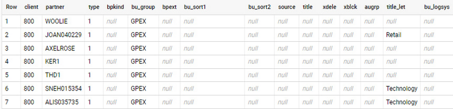
In an append-always replication in BigQuery, all updates are received as new records. For example, deleting a record in the source will be represented as a new record in BigQuery with a deletion flag. This applies to whether the records are coming from raw tables like BUT000 itself or pre-aggregated data, as from a BW extractor or a CDS view.

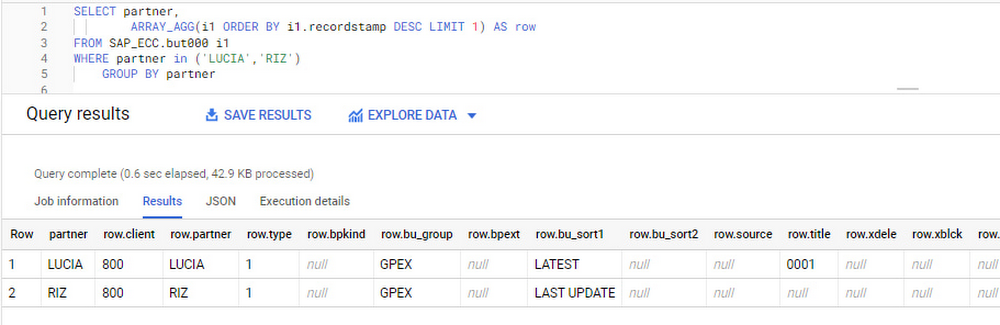
Let’s take a closer look at data coming particularly from the partners “LUCIA” and “RIZ”. The operation flag tells us whether the new record in BigQuery is an insert (I), update (U) or deletion (D), while the timestamps help us identify the latest version of our business partner.

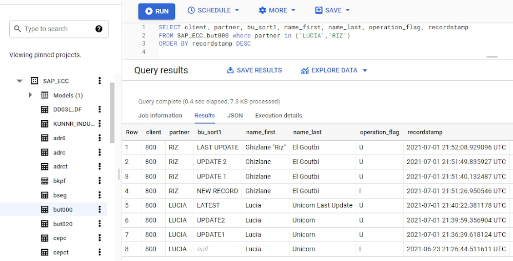
If we want to find the latest updated record for the partners LUCIA and RIZ, this is what the query would look like:

With the following result:

After identifying stale records for “LUCIA” and “RIZ” business partners, we can proceed to deleting all stale records for “LUCIA” if we do not want to retain the history. In this example, we are using a different table to which the same replication has been done, for the purpose of comparison and to check that all stale records have been deleted for the selection made and that we only kept last updated records. For example:

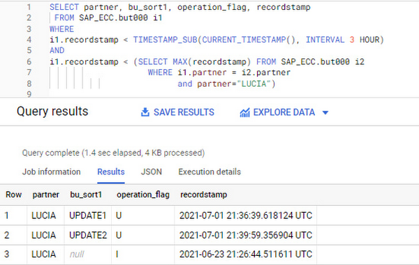
You can also use the following query to retrieve stale records for “LUCIA” partner before moving forward with deletion

Which produces all of the records, except the latest update:

Partitioning and clustering

To limit the number of records scanned in a query, save on cost and achieve the best performance possible, you’ll need to take two important steps: determine partitions and create clusters. 

Partitioning
A partitioned table is one that’s divided into segments, called partitions, which make it easier to manage and query your data. Dividing a large table into smaller partitions improves query performance and controls costs because it reduces the number of bytes read by a query.

You can partition BigQuery tables by:

• Time-unit column: Tables are partitioned based on a “timestamp,” “date,” or “datetime” column in the table.

• Ingestion time: Tables are partitioned based on the timestamp recorded when BigQuery ingested the data.

• Integer range: Tables are partitioned based on an integer column.

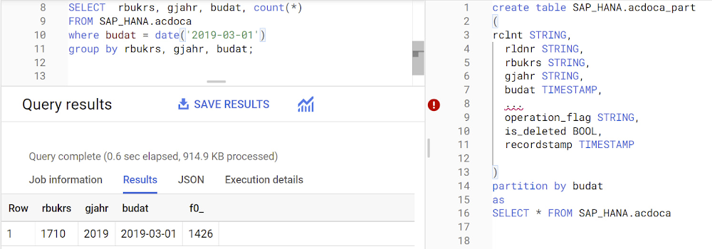
Partitions are enabled when the table is created, as in the example below.  A great tip is to always include the partition filter as shown on the left-hand side of the query.

Clustering
Clustering can be created on top of partitioned tables by applying the fields that are likely to be used for filtering. When you create a clustered table in BigQuery, the table data is automatically organized based on the contents of one or more of the columns in the table’s schema. The columns you specify are then used to colocate related data.

Clustering can improve the performance of certain query types — for example, queries that use filter clauses or that aggregate data. It makes a lot of sense to use them for large tables such as ACDOCA, the table for accounting documents in SAP S/4HANA. In this case, the timestamp could be used for partitioning, and common filtering fields such as the ledger, company code, and fiscal year could be used to define the clusters.

A great feature is that BigQuery will also periodically recluster the data automatically.

Materialized views

In BigQuery, materialized views are precomputed views that periodically cache the results of a query for better performance and efficiency. BigQuery uses precomputed results from materialized views and, whenever possible, reads only the delta changes from the base table to compute up-to-date results quickly. Materialized views can be queried directly or can be used by the BigQuery optimizer to process queries to the base table.

Queries that use materialized views are generally completed faster and consume fewer resources than queries that retrieve the same data only from the base table. If workload performance is an issue, materialized views can significantly improve the performance of workloads that have common and repeated queries. While materialized views currently only support single tables, they are very useful common and frequent aggregations like stock levels or order fulfillment.

Further tips on performance optimization while creating select statements can be found in the documentation for optimizing query computation.

Deployment pipeline and security

For most of the work you’ll do in BigQuery, you’ll normally have at least two delivery pipelines running — one for the actual objects in BigQuery and the other to keep the data staging, transforming, and updated as intended within the change-data-capture flows. Note that you can use most existing tools for your Continuous Integration / Continuous Deployment (CI/CD) pipeline — one of the benefits of using an open system like BigQuery. But, if your organization is new to CI/CD pipelines, this is a great opportunity to gradually gain experience. A good place to start is to read our guide for setting up a CI/CD pipeline for your data-processing workflow.  

When it comes to access and security, most end-users will only have access to the final version of the BigQuery views. While row and column-level security can be applied, as in the SAP source system, separation of concerns can be taken to the next level by splitting your data across different Google Cloud projects and BigQuery datasets. While it’s easy to replicate data and structures across your datasets, it’s a good idea to define the requirements and naming conventions early in the design process so you set it up properly from the start. 

Start driving faster and more insightful analytics

The best piece of advice we can give you is this: Try it yourself. Anyone with SQL knowledge can get started using the free BigQuery tier. New customers get $300 in free credits to spend on Google Cloud during the first 90 days. All customers get 10 GB storage and up to 1 TB queries/month, completely free of charge. In addition to discovering the massive processing capabilities, embedded machine learning, multiple integration tools, and cost benefits, you’ll soon discover how BigQuery can simplify your analytics tasks. 

If you need additional assistance, our Google Cloud Professional Services Organization (PSO) and Customer Engineers will be happy to help show you the best path forward for your organization. For anything else, contact us at cloud.google.com/contact.